A SQL crash course: the easiest way to gain an edge as a generalist in tech

Resource

Written by Sean Newman, mentor at The Commons.

‍

To get ahead, generalists need to learn to code. We’ve all heard this mantra in one form or another. The thing is, as a generalist, it’s less about technical expertise, and more about application. This means SQL is by far the language that will yield the best results for those in Biz Ops, Strategic Finance, Product, and Growth Marketing. Python is probably not going to help you in your day job as much.

Learning SQL and understanding its application is the quickest way to differentiate yourself from your peers. So what do I mean by application? Application means pulling together the right data (and summarizing it!) in such a way that you can make a strategic decision.

‍

‍

See what happened? This dramatically simplified example was possible because an all-star analyst did the following:

Defined the problem: Orders take too much time. He needed to find just how many minutes per order per courier.
Defined potential variables: Date, Time of Day, Rating, and Different Legs of the Trip are all important areas to explore
Wrote the code: We’ll dive into this shortly
Analyzed the results: The leg of the trip waiting at the restaurant is far too long!

Now, the manager and his analyst can brainstorm together why couriers wait so long at restaurants and what solutions they have to offer. This is all because the analyst not only knew how to write SQL (step 3), but also how to apply it (steps 1, 2, and 4). We’re going to look at everything you need to know for steps 3. But to take things to the next level, I recommend also finding opportunities at your job or in The Commons to work on real-world examples!

WHAT IS SQL?

Let’s first establish a few definitions…

Query = SQL code
Raw Data = An output table containing information specified by a query
Table = Database objects containing rows and columns of information
Schema: A collection of tables
Database: A collection of schemas

It’s important to understand how tables, schemas, and databases fit into an ecosystem. This will help you combine different datasets into the most meaningful raw data. Within schemas, each table is typically defined as “dim” or “fct”.

Dim stands for dimension. This is a static mapping table such as dim_quantities. It tells information about data. For example, dim_quantites may say the size of each package. Strawberries are 1.5 lbs, Oranges are 0.75 lbs, etc.
Fct stands for fact. These tables update in real time with activity such as purchases and inventory movement. For example, fct_groceries may say the time when each fruit was purchased by a customer

THE BASICS:

Every SQL statement should include the following attributes.

SELECT… determines which columns to include. This example has * which means every column in the table will be pulled in
FROM… determines which table to pull from. This example is pulling from a table called fct_groceries
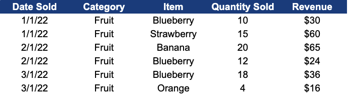
WHERE… determines how data should be filtered. This query specifies only the year 2022 and onward. It also excludes any row that is in a category outside of Fruits.

The output of this query is as follows. Since we selected * in the query above, it is showing us all of the data (both columns + rows) from the table.

Now, let’s build upon this query more…

We did a few new things here:

DATE_TRUNC… instead of individual days, we’ve bucketed the data into months (we always use the 1st of the month to do this). For example, 5/8/22 is now 5/1/22, or ‘2022-05-01’
COUNT… Each row counts as one. This is counting the rows within the unique combination of month_sold, category, and item. In layman's terms, this will tell us the total number of items sold each month.
SUM… this is summing the revenue for each sale within month_sold, category, and item. Similar to the above, this will tell us the total revenue by item, per month.
ORDER BY… this is always optional. ORDER BY sorts your data. In this example, the data is being sorted by month_sold, then by category, then by item in ascending order. By default, ORDER BY sorts the data in ascending order. To sort the data in descending order, use DESC - eg. ORDER BY [field names] DESC.
GROUP BY… when aggregations such as count or sum are included, “group by” always must be added at the end of the query. It’s very similar to the logic of a pivot table in Excel. The example below shows this. Notice how the two dark-yellow rows contain the same month, category, and item. They are combined and quantity_sold = 1 + 1, revenue = 3 + 3. When doing a GROUP BY, you can either number the columns chronologically as 1,2,3, or you can write out the column names as month, category, item.

Check out the new data set

If you’ve made it to this point, you now know enough SQL to be dangerous. Now, we’re going to go through other functions that are used on a daily basis by generalists making an impact at their companies!

INTERMEDIATE SQL:

This query creates the following table:

Don’t panic! A lot happened there, but we’re going to go through the changes in this query one by one.

Let’s start with “LEFT JOIN”.

‍

A JOIN is essentially the same as a VLOOKUP in Excel. Sometimes you need to access data that is stored in two separate tables. An easy way to do that is to use JOIN, which takes two tables with a shared column and combines them into a new table. In this case, fct_groceries (which I’ve nicknamed “g”) is being joined to dim_quantities (which I’ve nicknamed “q”). They both have a column named item, which if you recall can be blueberry, or strawberry, or orange.

The important thing with JOIN is first, to understand what the unique identifier is between tables. This is something that both tables share on the right level of granularity. The wrong level of granularity for example, category, will result in incorrect combinations.

The second piece is which type of JOIN to use. We performed a LEFT JOIN which is by default the safe option. This means every row of fct_groceries is still included and only the rows of dim_quanities that have a match in fct_groceries are included.

To reiterate, in the above example, I needed to combine fct_groceries with dim_quantities so I can figure out the weight of each fruit type. To do that I look at every row that shares a common item between each table. If they both contain “Orange” then the size in dim_quantities can be included with “orange” in the new table. Without all the extra functions above, this LEFT JOIN would give us the following information:

There are four main types of JOINs (although other lesser-used JOINs exist such as cross-join, but that is an advanced topic).

^{PHOTO SOURCE}

But what about that “CASE WHEN”?

‍

What about it, indeed? The great thing about SQL is it reads similar to the English language. A CASE WHEN is simply saying “for each row when ABC happens, do XYZ.”

In this case, when the item, which we’ve established is a type of fruit, is either Strawberry or Blueberry, then we rename it “Berry”. If not, (ELSE), we give it the original item name. The purpose of doing this here is to simplify the categorization so that we can work off of fewer buckets of data.

Every command written in blue in the CASE WHEN must be included for the query to work. You can also use multiple WHENs. Here’s an example:

A few miscellaneous call-outs

I renamed fct_groceries “g” (done in line 10) and every column from fct_groceries is now called g.category, or g.revenue. This is a good way to stay organized and easier than typing out fct_groceries every time. The same goes for dim_quantities as q (done in line 11).
“IN” and “=” are both ways to establish criteria. “=” works for one piece of criteria such as the ‘Plantains’ example. IN works for multiple criteria
Since we’re creating a new table, I always make sure my columns have a name. That way, when you’re looking at the output, you know what column is what. For example, I changed date_trunc('month',g.date_sold) to month_sold

THE FIRST STEP TO MASTERING SQL: SUBQUERIES

Finally, I want to get into the best SQL function out there. This takes a logical leap beyond what we’ve learned today, but it is a very powerful tool. Essentially, a subquery is a small table that is made and joined with the main table. Since databases are typically massive, it’s important to narrow down your search constraints to get a manageable raw data output.

I’ve decided to pivot to a more complicated data assessment than groceries for this example. If you recall the aforementioned Uber problem above, we were asked to figure out why our couriers are taking so long to deliver meals to people.

This table pulls primary from fct_deliveries which looks as follows without any edits:

It joins this table to ratings which is a subquery based on the table fct_ratings. This subquery looks as follows prior to being LEFT JOINed to the main table:

Remember, the value of subqueries is to minimize the lift of a data pull. This takes a lot less computing power than pulling directly from fct_ratings. You can pull multiple subqueries into a main query.

Side Note: you can see we’ve used the CASE WHEN logic to categorize the delivery_hour into Morning, Afternoon and Evening, so that we can simplify the data output. Rather than looking at 24 hours in a day, we’ve bucketed it into three time chunks that I’m hypothesizing to be relevant in this analysis.

You’ll also see a new function here, datediff. This simply calculates the time difference, in minutes (since “minutes'' the qualifier I used in the query), between two timestamps. You can see in row 15 that it’s calculating the time between when the order begins and when the courier comes to the restaurant. I’ve gone ahead and renamed each of the time buckets by using the “as'' function, so that I can clearly understand the output. For example, in row 15, I’ve named this time bucket minutes_to_order_pickup.

In this example, we’ve added a second sub-query which we’ve called courier_attributes. The courier_attributes table tells us the age_group and gender of each eater, which we can pull into our main table output. We now have a table that looks like this:

Notice how the tables were joined on delivery_id and courier_id. Now we have details such as age_group, gender, and rating. Each row represents a unique delivery. This is why some rows share the same date, courier_id, time_of_day, age_group, and gender. The only unique component is the delivery_id.

As I scan this raw data, it’s clear that deliveries with short minutes_at_restaurant have higher ratings. We would need to solidify this using statistics, but at a glance it appears that our final recommendation is to speed up the time couriers spend at restaurants waiting.

IN CONCLUSION:

We’ve learned SELECT, FROM, WHERE, CASE WHEN, LEFT JOIN, SUBQUERY and more in this SQL crash course. More importantly, we’ve learned how to apply this information to real-world business cases. There is a whole lot more to learn, but here’s a secret: googling is your friend! To this day, I google SQL functions all the time. I even had to google the syntax for “datediff” while writing this piece. Challenge yourself to figure out functions this way.

And remember, when your manager comes to you with a problem, think sequentially!

Define the problem
Define potential variables
Write the code
Analyze the results

That’s all I’ve got for now. It’s up to you to find meaningful ways to apply this information. The SQL muscle will grow and things will begin to click faster and faster over time. This knowledge doesn’t go away, and even provides value in senior positions. I’ll close with one more piece of monumentally important advice…

‍

It’s pronounced “see-quell” not “S-Q-L”!!!!

‍

Interested in flexing your SQL muscle? Join The Commons' Strategy & Operations Sprint to learn and apply SQL to a project similar to one you'd get in a Strategy & Operations role in tech.